![=]](/img/smile.svg)
Example Problems on Randomization
ST520 Homework 3 on Randomization
Problems: 1, 2, 3, 4
1
In a small clinical trial, permuted block randomization was used to assign one of two antiviral treatments (A or B) to eight patients with HIV disease. Four blocks of size 2 were chosen, each with one A and one B chosen at random. The endpoint of interest was change from baseline in log CD4 counts after eight weeks of treatment. The results of the trial are summarized as follows:
\[\begin{array}{c c c} & \rlap{\text{Block 1}} & \\ \hline \text{treatment} & \text{A} & \text{B} \\ \text{response} & 0.3 & 0.9 \\ \hline & \rlap{\text{Block 2}} & \\ \hline \text{treatment} & \text{B} & \text{A} \\ \text{response} & 1.0 & 0.2 \\ \hline & \rlap{\text{Block 3}} & \\ \hline \text{treatment} & \text{B} & \text{A} \\ \text{response} & 0.5 & 0.7 \\ \hline & \rlap{\text{Block 4}} & \\ \hline \text{treatment} & \text{A} & \text{B} \\ \text{response} & 0.1 & 0.2 \\ \hline \end{array}\]The test statistic used to evaluate whether treatment B has better response than treatment A is based on $\hat{Y_B}-\hat{Y_A}$, where $\hat{Y_B}$ is the average response among patients assigned to treatment B and $\hat{Y_A}$ is the average response for treatment A. We assume the sharp null hypothesis and reject in favor of treatment B if the test statistic is sufficiently large (i.e., one-sided test).
(a)
Find the distribution of the test statistic that is induced by the permuted block randomization under the sharp null hypothesis (i.e., design based inference).
To make find the distribution of the test statistic using permuted block randomization under the sharp null hypothesis, we need to find the average change in treatment response (in our case $B-A$) for all possible scenarios. Notice that we have 4 blocks of 2, so we have ${2 \choose 1}^4 = 16$ possible scenarios.
\[\begin{array}{| c | c c | c c | c c | c c | c c | c |} \hline i & \rlap{\text{Block 1}} & & \rlap{\text{Block 2}} & & \rlap{\text{Block 3}} & & \rlap{\text{Block 4}} & & & \bar{Y_B} & \bar{Y_A} & \bar{Y_B} - \bar{Y_A}\\ \hline & 0.3 & 0.9 & 1.0 & 0.2 & 0.5 & 0.7 & 0.1 & 0.2 & & & \\ 1 & A & B & B & A & B & A & A & B & & 0.65 & 0.325 & 0.325 \\ 2 & A & B & B & A & B & A & B & A & & 0.625 & 0.35 & 0.275 \\ 3 & A & B & B & A & A & B & A & B & & 0.7 & 0.275 & 0.425 \\ 4 & A & B & B & A & A & B & B & A & & 0.675 & 0.3 & 0.375 \\ 5 & A & B & A & B & B & A & A & B & & 0.45 & 0.525 & -0.075 \\ 6 & A & B & A & B & B & A & B & A & & 0.425 & 0.55 & -0.125 \\ 7 & A & B & A & B & A & B & A & B & & 0.5 & 0.475 & 0.025 \\ 8 & A & B & A & B & A & B & B & A & & 0.475 & 0.5 & -0.025 \\ 9 & B & A & B & A & B & A & A & B & & 0.5 & 0.475 & 0.025 \\ 10 & B & A & B & A & B & A & B & A & & 0.475 & 0.5 & -0.025 \\ 11 & B & A & B & A & A & B & A & B & & 0.55 & 0.425 & 0.125 \\ 12 & B & A & B & A & A & B & B & A & & 0.525 & 0.45 & 0.075 \\ 13 & B & A & A & B & B & A & A & B & & 0.3 & 0.675 & -0.375 \\ 14 & B & A & A & B & B & A & B & A & & 0.275 & 0.7 & -0.425 \\ 15 & B & A & A & B & A & B & A & B & & 0.35 & 0.625 & -0.275 \\ 16 & B & A & A & B & A & B & B & A & & 0.325 & 0.65 & -0.325 \\ \hline \end{array}\](b)
What is the p-value for the clinical trial described above?
We want to use a one sided p-value since we are testing if B is better than A. Under the sharp null hypothesis is our p-value is the total number of $t_i$’s greater than or equal to $t_1$ divided by the total number of trials. Notice that only trial 1, 3, and 4, meet this criteria. Thus,
\[p = P(T \geq t_1 | \text{ sharp } H_0) = \frac{ 3 }{ 16 } = 0.1875.\](c)
What are the advantages and disadvantages of this kind of design as compared to using simple randomization where each treatment is assigned with probability of half independently of each other?
With simple randomization, there is a fairly high change of imbalanced groups, especially with smaller sample sizes. Permuted block randomization solves that by ensuring that the groups are balanced (with at most $\frac{ block size }{ 2 }$ imbalance). However, this study does not using a varying block size. Thus, when the first patient in the block is assigned a treatment, the treatment for the other person is known (to be the other treatment). This may introduce other biases.
2
Let the random variable $X\sim b(n,\pi)$. The sample proportion is denoted by $p=X/n$.
(a)
Prove that
\[\Big( \frac{ n }{ n-1 } \Big) p (1-p)\]is an unbiased estimator for $\pi(1-\pi), \ n \geq 2$.
\[\begin{align} E\Big(\frac{ n }{ n-1 }\cdot p (1-p)\Big) & = \frac{ n }{ n-1 }E(\frac{ X }{ n } ( 1- \frac{ X }{ n })) \\ & = \frac{ n }{ n-1 } E(\frac{ X }{ n } - \frac{ X^2 }{ n^2 }) \\ & = \frac{ n }{ n-1 } \Big( \frac{ 1 }{ n } E(X) - \frac{ 1 }{ n^2 }E(X^2) \Big) \\ & = \frac{ n }{ n-1 } \Big( \frac{ 1 }{ n } (n \cdot \pi) - \frac{ 1 }{ n^2 }(n\cdot \pi(1-\pi) + n^2 \pi^2) \Big) \\ & = \frac{ n }{ n-1 } \Big( \pi - \frac{ 1 }{ n^2 } (n \pi - n \pi^2 + n^2 \pi^2) \Big) \\ & = \frac{ n }{ n-1 } \Big( \pi - \frac{ \pi }{ n } + \frac{ \pi^2 }{ n } - \pi^2 \Big) \\ & = \frac{ n \pi - \pi + \pi^2 - n \pi^2 }{ n - 1 } \\ & = \frac{ \pi (n-1) - \pi^2(n-1) }{ n = 1 } \\ & = \pi - \pi^2 \\ & = \pi (1-\pi) \end{align}\](b)
Consider data from $N$ studies using the same treatment regimen. We observe $(X_i, n_i), \ i = 1, \dots, N$, where $n_i$ denotes the number of patients in the $i$-th study and $X_i$ denotes the number of these patients that respond to treatment. It will be assumed that these data are from a hierarchical model where $(X_i, n_i, \pi_i), \ i = 1, \dots, N$ are assumed to be iid random vectors. The $\pi_i$ are assumed to be study-specific response rates which themselves represent an iid sample from some distribution. Conditional on $\pi_i$ and $n_i$, $X_i$ is assumed to follow a binomial distribution. Specifically,
\[X_i | n_i, \ \pi_i \sim b(n_i, \pi_i).\]Find an unbiased estimator for the expectation
\[E[\pi_i (1-\pi_i)]\]and prove that is unbiased.
\[\begin{align} E \Big[ E\Big( \frac{ n_i }{ n_i - 1 } \cdot p_i (1-p_i) \Big) \Big] & = E \Big[ E\Big( \frac{ n_i }{ n_i - 1 } \cdot \frac{ X_i }{ n_i } (1-\frac{ X_i }{ n_i }) \Big) \Big] \\ & = E \Big[ \frac{ 1 }{ n_i - 1 } \cdot E\Big( X_i - \frac{ X_i^2 }{ n_i } \Big) \Big] \\ & = E \Big[ \frac{ 1 }{ n_i - 1 } \cdot \Big( E(X_i) - E\Big(\frac{ X_i^2 }{ n_i }\Big) \Big) \Big] \\ & = E \Big[ \frac{ 1 }{ n_i - 1 } \cdot \Big( E(E(X_i | n_i, \pi_i )) - \frac{ 1 }{ n_i } E(E(X_i^2 | n_i, \pi_i )) \Big) \Big] \\ & = E \Big[ \frac{ 1 }{ n_i - 1 } \cdot \Big( E(n_i \pi_i) - \frac{ 1 }{ n_i } E(n_i \pi_i (1-\pi_i) + n_i^2 \pi_i^2) \Big) \Big] \\ & = E \Big[ \frac{ 1 }{ n_i - 1 } \cdot \Big( E(n_i \pi_i) - \frac{ 1 }{ n_i } E(ni_i \pi_i - n_i \pi_i^2 + n_i^2 \pi_i^2) \Big) \Big] \\ & = E \Big[ \frac{ 1 }{ n_i - 1 } \cdot \Big( E(n_i \pi_i) - E( \pi_i - \pi_i^2 + n_i \pi_i^2 \Big) \Big] \\ & = E \Big[ \frac{ 1 }{ n_i - 1 } E(n_i \pi_i - \pi_i - \pi_i^2 + n_i \pi_i^2 \Big) \Big] \\ & = E \Big[ \frac{ n_i \pi_i - \pi_i + \pi_i^2 - n_i \pi_i^2 }{ n_i - 1 } \Big] \\ & = E \Big[ \frac{ \pi_i ( n_i - 1) + \pi_i^2(n_i - 1) }{ n_i - 1 } \Big] \\ & = E(\pi_i - \pi_i^2) \\ & = E(\pi_i ( 1 - \pi_i)) \end{align}\]3
Consider the following hierarchical model which may be appropriate in conceptualizing results from different studies using the same regimen but where the response of interest is a continuous measurement. The data from $N$ such studies are defined as
\[\{ (Y_{ij}, \ j=1, \dots, n_i), \ i=1, \dots, N \},\]where $Y_{ij}$ denotes the response from the $j$-th individual (among $n_i$ individuals) in the $i$-th study. The underlying hierarchical model assumes that there exists $N$ iid random vectors
\[\{ (Y_{ij}, \ j=1, \dots, n_i), \ \mu_i, \ \sigma_i^2 \}\]for $i = 1, \dots, N$. The random vectors $(\mu_i, \sigma_i^2), \ i = 1, \dots, N$ are themselves assumed to be iid unobserved random effects corresponding to the study specific mean and variance of response which are allowed to vary according to some distribution. In particular, we will denote the expected value of the study-specific means by
\[\mu^* = E(\mu_i)\]and the variance of the study-specific means by
\[\sigma_{*\mu}^2=var(\mu_i).\]Conditional on $\mu_i, \sigma_i^2, n_i$, we will assume the data from the $i$-th study represent $n_i$ iid observations with mean $\mu_i$ and variance $\sigma_i^2$. Specifically, we assume that for the $i$-th study
\[E(Y_{ij} | \mu_i, \sigma_i^2, n_i) = \mu_i, \ var(Y_{ij} | \mu_i, \sigma_i^2, n_i) = \sigma_i^2, \ j = 1, \dots , n\]The major reason for this conceptualization is to determine whether study to study variant in the mean response is substantial. Specifically, we want to estimate $\sigma_{*\mu}^2=var(\mu_i)$. In the table below, we summarize results from ten studies. For each study $i = 1, \dots , 10$, we give the sample size $n_i$, the sample mean response
\[\bar{Y_i}=\frac{ \sum^{n_i}_{j=1} Y_{ij} }{ n_i }\]and the sample variance
\[s_i^2 =\frac{ \sum^{n_i}_{j=1} (Y_{ij}- \bar{Y_i})^2 }{ n_i -1 }.\] \[\begin{array}{c c c c} \hline \text{study number} & \text{sample mean} & \text{sample variance} & \text{sample size} \\ \hline 1 & 59 & 2475 & 52 \\ 2 & 23 & 1971 & 48 \\ 3 & 41 & 2009 & 47 \\ 4 & 28 & 1771 & 163 \\ 5 & 40 & 2484 & 135 \\ 6 & 31 & 2139 & 150 \\ 7 & 34 & 2275 & 37 \\ 8 & 20 & 1411 & 111 \\ 9 & 30 & 2379 & 62 \\ 10 & 25 & 1622 & 100 \end{array}\](a)
In terms of $(\bar{Y_i}, s_i^2, n_i), \ i=1, \dots, N$ derive an unbiased estimator for $\sigma^2_{*\mu}$.
We can use the law of iterated expectation of variances.
\[\begin{align} Var(\bar{Y_i}) & = Var(E(\bar{Y_i} | \mu_i, \sigma_i^2)) + E(Var(\bar{Y_i} | \mu_i, \sigma^2_i))\\ & = Var(\mu_i) + E(\frac{ \sigma^2_i }{ n_i }) \\ & = \sigma_{*\mu}^2 + E(\frac{ \sigma^2_i }{ n_i }) \\ \sigma_{*\mu}^2 & = Var(\bar{Y_i}) - E(\frac{ \sigma^2_i }{ n_i }) \\ & = \frac{ 1 }{ N - 1 } \sum (\bar{Y_i} - \bar{\bar{Y}})^2 - \frac{ 1 }{ N } \sum \frac{ \sigma_i^2 }{ n_i } \end{align}\]Where $\bar{\bar{Y}}$ is the average of the means.
(b)
Derive this estimate for the data provided in the table above.
Notice that $\bar{\bar{Y}} = 33.1$.
\[\frac{1}{10-1} \cdot (20-33.1)^2+(23-33.1)^2+(25-33.1)^2+(28-33.1)^2+(30-33.1)^2+(31-33.1)^2+(34-33.1)^2+(40-33.1)^2+(41-33.1)^2+(59-33.1)^2 -\frac{1}{10} \left(\frac{2475}{52}+\frac{1971}{48}+\frac{2009}{47}+\frac{1711}{163}+\frac{2484}{135}+\frac{2139}{150}+\frac{2275}{37}+\frac{1411}{111}+\frac{2379}{62}+\frac{1622}{100}\right) = 98.6539\]4
Suppose the goal of a clinical trial is to estimate the difference in mean response between two treatments assumed to have the same variance. It costs 150 dollars to treat a patient on regimen A and 100 dollars to treat a patient on regimen B. An investigator has 30,000 dollars to spend on this trial.
(a)
What is the optimal allocation of patients to treatment A and B subject to the budgetary constraints of the investigator? That is, what allocation of patients would result in the smallest variance of the estimator of treatment difference?
Notice that we want to estimate and optimize $\Delta$, so we can use the equation,
\[\hat{\Delta} = \bar{Y_A} - \bar{Y_B} = \sigma^2 \Big( \frac{ 1 }{ n_A } + \frac{ 1 }{ n_B } \Big).\]Our optimization equation is $150 n_a + 100 n_b \leq 30000$. We can solve this for $n_B$ to get
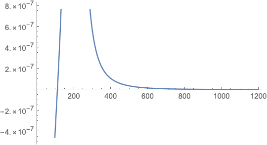
\[n_B = \frac{ 30000 - 150n_A }{ 100 }.\]We can then plug this into the equation for $\hat{\Delta}$ and take the derivative at 0 to find where the variance is minimized.
\[\begin{align} \hat{\Delta} & = \sigma^2 \Big( \frac{ 1 }{ n_A } + \frac{ 100 }{30000 - 150n_A } \Big)\\ \frac{ d }{ dn_A }\hat{\Delta} & = \frac{ 15000 \sigma^2 }{ (30000-150\cdot n_A)^2 } - \frac{ \sigma^2 }{ n_A^2 } \\ 0 & = \frac{ 15000 \sigma^2 }{ (30000-150\cdot n_A)^2 } - \frac{ \sigma^2 }{ n_A^2 } \\ n_A & = 110.102, 1089.9 \end{align}\]We see on the graph that the derivative goes from negative to positive at 110.102, so we will examine that point further. Also notice that 1089.9 lives outside of the budget constraint.
Since our $n_A$ is not a whole number, we will check both 110 and 111 to see which gives the lowest variance.
\[\begin{align} @ n_A = 110 \\ n_B & = \frac{ 30000-150(110) }{ 100 } \\ & = 135 \\ \hat{\Delta} & = \sigma^2 \Big( \frac{ 1 }{ 110 } + \frac{ 1 }{ 135 } \Big)\\ & = 0.0164983 \sigma^2 \end{align}\] \[\begin{align} @ n_A = 111 \\ n_B & = \frac{ 30000-150(111) }{ 100 } \\ & = 133.5 = 133 & \text{round down due to budget} \\ \hat{\Delta} & = \sigma^2 \Big( \frac{ 1 }{ 111 } + \frac{ 1 }{ 133 } \Big)\\ & = 0.0165278 \sigma^2 \end{align}\]We can see that the case $n_A = 110, \ n_B = 0.164983$ gives the lowest variance, thus it is the optimal allocation.
(b)
If the investigator insisted on equal allocation to both treatments, then how much more money would need to be spent to get the same degree of precision (i.e. variance of estimator) as the allocation in part (a).
Equal treatments means that $n_A = n_B$. In order to have the same variance,
\[\begin{align} 0.0164983 \sigma^2 & = \sigma^2 (\frac{ 1 }{ n_A } + \frac{ 1 }{ n_B })\\ & = \sigma^2 (\frac{ 1 }{ n_A } + \frac{ 1 }{ n_A })\\ n_A & = \frac{2}{.0164717}. \end{align}\]For the sake of having the exact same variance, we will leave this unrounded. Thus, the investigator would need to spend
\[\begin{align} \text{Budget} & = 150 \cdot \frac{2}{.0164717} + 100 \cdot \frac{2}{.0164717} \\ & = 30355.1\\ \end{align}\]This is $30000 - 30355.1 = 355.10$ dollars more than the imbalanced study.