• 2.1
• 2.2
  • a.
  • b.
• 2.3
  • a.
  • b.
  • c.
• 2.9
• 2.16
• 2.22 (part a)
  • a

2.1

Let $Y_1, \dots, Y_n$ be iid positive random variables such that $Y^{(\lambda)}$ is assumed to have a normal$(\mu, \sigma^2)$ distributions where

\[Y^{(\lambda)} = \begin{cases} \frac{ Y^\lambda -1 }{ \lambda } & \text{when } \lambda \neq 0 \\ \log(Y) & \text{when } \lambda = 0 \end{cases}\]

(The normality assumption is actually only possible for $\lambda = 0$, but ignore that detail.) Derive the log likelihood $\ell_n (\mu, \sigma, \lambda | \mathbf Y)$ of the observed data $Y_1, \dots, Y_n$. Note that $y^{(\lambda)}$ is a strictly increasing function of $y$ (the derivative is always positive). It might be easiest to use the “distribution funtion” method to get the density of $Y_i$, but feel free to use Jacobians, etc.

We know $f_Y(y) = f_{y^{(\lambda)}}(y^{(\lambda)}) \cdot \frac{ d Y^{(\lambda)} }{ dY }$ (the CDF method). We will find this piecewise and then combine it into a likelihood.

\[\frac{ d Y^{(\lambda)} }{ dY } = \begin{cases} Y^{\lambda - 1} & \lambda \neq 0 \\ \frac{ 1 }{ Y } & \lambda = 0 \end{cases}\]

Notice that in the second case $1/Y = Y^{\lambda - 1}$ since $\lambda = 0$.

\[f_Y(y) = \begin{cases} y^{\lambda - 1} \frac{ 1 }{ \sqrt{ 2 \pi \sigma^2 }} \exp \Big\{ -\frac{ 1 }{ 2 \sigma^2 }(\frac{ y^\lambda -1 }{ \lambda }- \mu)^2 \Big\} & \lambda \neq 0\\ y^{\lambda - 1} \frac{ 1 }{ \sqrt{ 2 \pi \sigma^2 }} \exp \Big\{ -\frac{ 1 }{ 2 \sigma^2 }(\log(y)- \mu)^2 \Big\} & \lambda = 0 \end{cases}\]

Now we can combine them using an indicator into a likelihood function.

\[\begin{align} L(\mu, \sigma, \lambda | Y) & = \prod_{i=1}^n f_Y(y_i) \\ & =\prod_{i=1}^n y_i^{\lambda - 1} \frac{ 1 }{ \sqrt{ 2 \pi \sigma^2 }} \exp \Big\{ -\frac{ 1 }{ 2 \sigma^2 }(\frac{ y_i^\lambda -1 }{ \lambda }- \mu)^2 \Big\} \mathbb I(\lambda \neq 0) \\ & \times y_i^{\lambda - 1} \frac{ 1 }{ \sqrt{ 2 \pi \sigma^2 }} \exp \Big\{ -\frac{ 1 }{ 2 \sigma^2 }(\log(y_i)- \mu)^2 \Big\} \mathbb I(\lambda = 0) \\ & = \prod_{i=1}^n y_i^{\lambda - 1} \frac{ 1 }{ \sqrt{ 2 \pi \sigma^2 } } \\ & \times \exp \Big\{ - \frac{ 1 }{ 2 \sigma^2 } \Big( (\frac{ y_i^\lambda -1 }{ \lambda }- \mu)^2 \mathbb I( \lambda \neq 0 )+ (\log(y_i)- \mu)^2 \mathbb I( \lambda = 0 ) \Big) \Big\} \\ & = y_i^{ n(\lambda - 1)} (2 \pi \sigma^2)^{-n/2} \\ & \times \exp \Big\{ - \frac{ 1 }{ 2 \sigma^2 } \Big( \sum_{i=1}^n (\frac{ y_i^\lambda -1 }{ \lambda }- \mu)^2 \mathbb I( \lambda \neq 0 )+ \sum_{i=1}^n (\log(y_i)- \mu)^2 \mathbb I( \lambda = 0 ) \Big) \Big\} \\ \ell(\mu, \sigma, \lambda | Y) &= (\lambda - 1)\sum_{i=1}^n \log(y_i) - \frac{ n }{ 2 } \log(2 \pi \sigma^2)\\ & - \frac{ 1 }{ 2 \sigma^2 } \Big[ \sum_{i=1}^n (\frac{ y_i^\lambda -1 }{ \lambda }- \mu)^2 \mathbb I( \lambda \neq 0 )+ \sum_{i=1}^n (\log(y_i)- \mu)^2 \mathbb I( \lambda = 0 ) \Big] \end{align}\]

2.2

One of the data sets obtained from the 1984 consulting session on max flow of rivers was $n=35$ yearly maxima from one station displayed in the following R printout.

a.

Find the maximum likelihood estimates for the extreme value location-scale density $f(y; \mu, \sigma) = f_0((y-\mu)/\sigma)/\sigma$, where

\[f_0(t)=e^{-t}e^{-e^{-t}}.\]

Before coding this up to find the MLEs, we need to find the log-likelihood.

\[\begin{align} L(\mu, \sigma | Y) & = \prod_{i=1}^n f_0(\frac{ y-\mu }{ \sigma })/\sigma \\ & = \frac{ 1 }{ \sigma^n } \prod_{i=1}^n e^{-\frac{ y_i - \mu }{ \sigma }} \exp(-e^{-\frac{ y_i - \mu }{\sigma}}) \\ \\ \ell(\mu, \sigma | Y ) & = -n \log(\sigma) + \sum_{i=1}^n (\frac{ -y_i + \mu }{ \sigma }) - \sum_{i=1}^n \exp(\frac{ -y_i + \mu }{\sigma}) \\ \end{align}\]

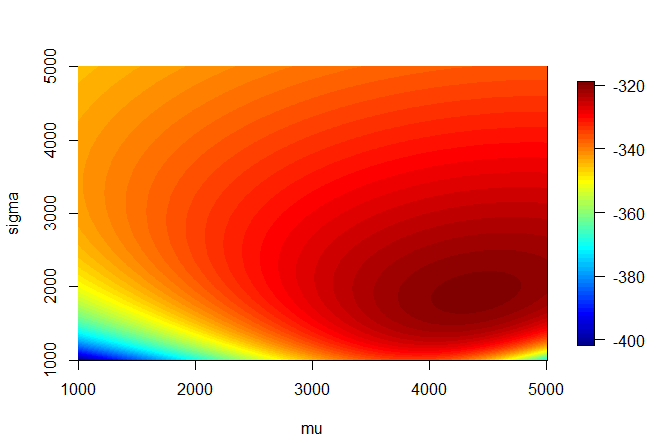
We would expect our estimates to lie in the dark red region of this heatmap.

Our estimates are $\mu = 4395.147$ and $\sigma = 1882.499$. These are where we would expect from our heatmap. These values also seemed invariant to different starting values after a few tests.

b.

Draw a QQ plot and the parametrically estimated distribution function overlaid with the empirical distribution function.

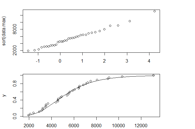
Our QQ Plot looks like a straight line, which means we have a good estimate. Also the CDF follows the data fairly well.

2.3

Recall the ZIP model

\(\begin{align} P(Y = 0) & = p + (1-p) e^{-\lambda} \\ P(Y = y) & = (1-p) \frac{ \lambda^y e^{-\lambda} }{ y! } & y = 1, 2, \dots \end{align}\)

a.

Reparameterize the model by defining

\[\pi \equiv P(Y = 0) = p + (1-p)e^{-\lambda}.\]

Solve for $p$ in terms of $\lambda$ and $\pi$, and then substitute so that the density depends on only $\lambda$ and $\pi$.

\[\begin{align} \pi & = p + (1-p)e^{-\lambda} \\ \pi & = p + e^{-\lambda} - p e^{-\lambda} \\ \pi - e^{-\lambda} & = p (1 - e^{-\lambda}) \\ \frac{ \pi - e^{-\lambda} }{ 1 - e^{-\lambda} }& = p \end{align}\] \[F_Y(y; \pi, \lambda) = \begin{cases} \pi & y = 0\\ \Big( 1 - \frac{ \pi - e^{-\lambda} }{ 1 - e^{-\lambda} } \Big) \frac{ e^{-\lambda} \lambda^y }{ y! } & y = 1, 2, \dots \end{cases}\]

b.

For an iid sample of sample of size $n$, let $n_0$ be the number of zeroes in the sample. Assuming that the complete data is available (no grouping), show that the likelihood factors into two pieces and that $\widehat \pi = n_0 / n$ (This illustrates why we obtained exact fits for the 0 cell in Example 2.1 p 32.) Also show that the maximum likelihood estimator for $\lambda$ is the solution to a simple nonlinear equation involving $\overline{ Y_+ }$ (the average of the nonzero values).

\[\begin{align} L(\lambda, \pi | Y) & = \prod_{i=1}^n f_Y(y_i) \\ & = \pi^{n_0} \Big[ \Big( 1 - \frac{ \pi - e^{-\lambda} }{ 1 - e^{-\lambda} } \Big) e^{-\lambda}\Big]^{n-n_0} \prod_{Y_i > 0} \frac{ \lambda^{y_i} }{ y_i ! } \\ \ell(\lambda, \pi | Y) & = n_0 \log(\pi) + (n - n_0) \Big[ \log\Big( 1 - \frac{ \pi - e^{-\lambda} }{ 1 - e^{-\lambda} } \Big) - \lambda\Big] + \sum_{Y_i > 0} y_i \log(\lambda) - \log(y_i!) \\ \\ \frac{ \partial \ell }{\partial \pi} & = \frac{ n_0 }{ \pi } -\frac{ n - n_0 }{ 1 - \pi } + 0 \stackrel{\text{set}}{=}0\\ 0 & = \frac{ n_0( 1-\widehat\pi) - \widehat\pi(n-n_0) }{ \widehat\pi (1-\widehat\pi) } \\ \widehat\pi = \frac{ n_0 }{ n } \\ \\ \frac{ \partial \ell }{\partial \lambda } & = 0 + \frac{ e^\widehat\lambda(-n + n_0) }{ -1 + e^\widehat\lambda } + \sum_{y_i > 0} \frac{ y_i }{ \widehat\lambda } \stackrel{\text{set}}{=}0 \\ \frac{ e^\widehat\lambda(-n + n_0) }{ -1 + e^\widehat\lambda } & = - \sum_{y_i > 0} \frac{ y_i }{ \widehat\lambda } \\ \frac{ \widehat\lambda }{ 1 - e^{-\widehat\lambda} } & = \overline{ Y }_+ \end{align}\]

c.

Now consider the truncated or conditional sample consisting of the $n-n_0$ nonzero value. Write down the conditional likelihood for these values and obtain the same equation for $\hat \lambda_{MLE}$ as in a). (First write down the conditional density of $Y$ given $Y > 0$.)

Instead of a Zero Inflated Poisson, we are now dealing with a Zero Truncated Poisson.

\[g(y ; \lambda) = P(Y = y | Y > 0) = \frac{ f(y; \lambda) }{ 1- f(0; \lambda) } = \frac{ \lambda^y e^{-\lambda} }{ y! (1-e^{-\lambda}) } = \frac{ \lambda^y}{ y!(e^\lambda - 1) }\]

We can now find the MLE using this PDF.

\[\begin{align} L(\lambda | Y) & = \prod_{i=1}^{n-n_0} g(y; \lambda) \\ & = \prod_{i=1}^{n-n_0} \frac{ \lambda^{y_i}}{ y_i!(e^\lambda - 1) } \\ \ell(\lambda | Y) & = \sum_{i=1}^{n-n_0} y_i \log(\lambda) - \log(y_i!) - \log(e^\lambda - 1) \\ \frac{ \partial \ell }{\partial \lambda} & = \frac{ \sum y_i }{ \lambda } - 0 - \frac{ (n-n_0) e^\lambda }{ e^\lambda - 1} \stackrel{\text{set}}{=}0 \\ \frac{ \widehat\lambda }{ 1 - e^{-\widehat\lambda} } & = \overline{ Y }_+ \end{align}\]

2.9

The sample $Y_1, \dots , Y_n$ is iid with distribution function

\[F_Y(y; p_0, p_1, \alpha, \beta) = p_0 I(0 \leq y) + (1 - p_0 - p_1) F(y ; \alpha, \beta) + p_1 I(y \geq 1).\]

where $F(y; \alpha, \beta)$ is the beta distribution. You may recall that the beta density is positive on $0 < y< 1$ so that $F(0; \alpha, \beta) = 0$ and $F(1; \alpha , \beta) = 1$,

but otherwise you do not need to use or know its form in the following; just use $F(y; \alpha, \beta)$ or $f(y; \alpha, \beta)$ where needed. The physical situation relates to test scores standardized to lie in $[0,1]$, but where $n_0$ of the sample values are exactly 0 (turned into a blank test), $n_1$ values are 1 (a perfect score), and the rest are in between 0 and 1. Use the $2h$ method to show that the likelihood is

\[p_0^{n_0}p_1^{n_1}(1 - p_0 - p_1)^{n-n_0-n_1} \prod_{0 < Y_i<1} f(Y_i; \alpha, \beta).\]

Take $\theta = (p_0, p_1, \alpha, \beta)$

\[\begin{align} L(p_0, p_1, \alpha, \beta | y) & = \prod_{i=1}^n f_Y(y_i; \theta) \\ & = \lim_{h\rightarrow 0^+} \prod_{i=1}^n \frac{ 1 }{ 2 h } (F_Y(Y_i+h; \theta) - F_Y(Y_i - h; \theta)) \\ & = \lim_{h \rightarrow 0^+} \Big[ F_Y(0+h| \theta) - F_Y(0-h|\theta) \Big]^{n_0} \\ & \times \lim_{h \rightarrow 0^+} \Big[ F_Y(1+h| \theta) - F_Y(1-h|\theta) \Big]^{n_1} \\ & \times \lim_{h \rightarrow 0^+} \prod_{0 \leq Y_i \leq 1} \frac{ 1 }{ 2h } (F_Y(Y_i+h; \theta) - F_Y(Y_i-h; \theta)) \\ & = \Big[ p_0 + (1-p_0-p_1) F(h; \alpha, \beta) \Big]^{n_0} \Big[ p_1 + (1-p_0-p_1) F(1-h; \alpha, \beta) \Big]^{n_1} \\ & \times \lim_{h \rightarrow 0^+} \prod_{0 \leq Y_i \leq 1} \frac{ 1 }{ 2h } (1- p_0 - p_1) (F(Y_i+h; \theta) - F(Y_i-h; \theta)) \\ & = p_0^{n_0} p_1^{n_1} (1-p_0-p_1)^{n-n_0-n_1} \prod_{0 \leq Y_i \leq 1} f(Y_i; \alpha, \beta) \end{align}\]

2.16

The standard Box-Cox regression model (Box and Cox 1964) assumes that after transformation of the observed $Y_i$ to $Y^{(\lambda)}$ we have the linear model

\[Y_i^{(\lambda)} = x_i^T \beta + e_i,\ i = 1, \dots , n.\]

where $Y_i$ is assumed positive and the $x_i$ are known constants, $i = 1, \dots , n$. In addition assume that $e_1, \dots , e_n$ are iid normal$(0, \sigma^2)$ errors. Recall that the Box-Cox transformation is defined in Problem 2.1 (p.107) and is strictly increasing for all $\lambda$. Show that the likelihood is

\[L(\beta, \sigma, \lambda | \{ Y_i, x_i\}^n_{i=1} ) = \Big( \frac{ 1 }{ \sqrt{ 2 \pi \sigma^2 }} \Big)^n \exp \Big[ - \sum_{i=1}^n \frac{ (Y_i^{(\lambda)} - x_i^T \beta)^2 }{ 2 \sigma^2 } \Big] \times \prod_{i=1}^n \Bigg\lvert \frac{ \partial t^{(\lambda)} }{\partial t} \Big\rvert_{t=Y_i} \Bigg\rvert.\]

Notice that this situation is just a special case of the Box-Cox transformation. Instead of $\mu$, we have a specific mean, $Y_i^{(\lambda)} \sim N(x_i^T \beta, \sigma^2)$. As shown in 2.1, our likelihood will be

\[\begin{align} L(\beta, \sigma, \lambda | \{ Y_i, x_i\}^n_{i=1} ) & = \Big( \frac{ 1 }{ \sqrt{ 2 \pi \sigma^2 }} \Big)^n \exp \Big[ - \sum_{i=1}^n \frac{ (Y_i^{(\lambda)} - \mu)^2 }{ 2 \sigma^2 } \Big] \times \prod_{i=1}^n \Bigg\lvert \frac{ \partial t^{(\lambda)} }{\partial t} \Big\rvert_{t=Y_i} \Bigg\rvert \\ & = \Big( \frac{ 1 }{ \sqrt{ 2 \pi \sigma^2 }} \Big)^n \exp \Big[ - \sum_{i=1}^n \frac{ (Y_i^{(\lambda)} - x_i^T \beta)^2 }{ 2 \sigma^2 } \Big] \times \prod_{i=1}^n \Bigg\lvert \frac{ \partial t^{(\lambda)} }{\partial t} \Big\rvert_{t=Y_i} \Bigg\rvert. \end{align}\]

2.22 (part a)

Consider the standard one-way ANOVA situation with $Y_{ij}$ distributed as $N(\mu_i, \sigma^2), \ i = 1, \dots, k, \ j = 1, \dots, n_i$, and all the random variables are independent.

a

Form the log likelihood, take derivatives, and show that the MLEs are

$\widehat\mu_i = \overline{ Y }_i, \ i = 1, \dots k,$

$\widehat\sigma^2 = SSE/ N$

where $SSE = \sum_{i=1}^{k} \sum_{j=1}^{n_i} \Big( Y_{ij} - \overline{ Y }_i \Big)^2$

and $N = \sum_{i=1}^{k} n_i$.

\[\begin{align} L(\mu, \sigma^2 | y ) & = \prod_{i=1}^{k} \prod_{j=1}^{n_i} f(y_{ij}; \mu, \sigma) \\ & = \prod_{i=1}^k (2 \pi \sigma^2)^{-n_i/2} exp{\frac{ -1 }{ 2\sigma^2 } \sum_{j=1}^{n_i}(y_{ij} - \mu_i)^2 } \\ \ell (\mu, \sigma^2 | y) & = \sum_{i=1}^k \frac{ -n_i }{ 2 } \log(2 \pi \sigma^2) - \frac{ 1 }{ 2\sigma^2 }\sum_{j=1}^{n_i}(y_{ij} - \mu_i)^2 \\ & = \sum_{i=1}^k \frac{ -n_i }{ 2 } \log(2 \pi \sigma^2) - \frac{ 1 }{ 2\sigma^2 }\sum_{j=1}^{n_i}(y_{ij}^2 - 2 y_{ij} \mu_i + \mu_i^2) \\ \frac{ \partial \ell }{\partial \mu_a} & = -\frac{ 1 }{ 2 \sigma^2 }(0 - 2 \sum_{i=1}^{n_a} y_i + 2 n_a \mu_a) \stackrel{\text{set}}{=}0 \\ \widehat\mu_a & = \frac{ \sum_{i=1}^{n_a} y_i }{ n_a } \\ & = \overline{ Y }_a \\ \frac{ \partial \ell }{\partial \sigma^2} & = \sum_{i=1}^k \frac{ -n_i }{ 2 \sigma^2 } + \frac{ 1 }{ 2 (\sigma^2)^2} \sum_{j=1}^{n_i} (y_{ij} - \widehat \mu_i)^2 \stackrel{\text{set}}{=}0 \\ 0 & = \frac{ -N }{ 2 \sigma^2} + \frac{ 1 }{ 2 (\sigma^2)^2} \sum_{i=1}^{k} \sum_{j=1}^{n_i} (y_{ij} - \overline{ Y }_i)^2 \\ \frac{ N }{ 2 } \widehat\sigma^2 & = \frac{ 1 }{ 2 } SSE \\ \widehat\sigma^2 = \frac{ SSE }{ N } \end{align}\]

We can also check our second order conditions to ensure that this is a maximum.

\[\begin{align} \frac{ \partial^2 \ell }{\partial \mu_a^2} & = \frac{ -1 }{ \sigma^2 } < 0 \\ \frac{ \partial^2 \ell }{\partial (\sigma^2)^2}|_{\sigma^2 = \widehat\sigma^2} & = \frac{ N }{ 2 (\widehat\sigma^2)^2 }+ \frac{ SSE }{ (\widehat \sigma^2)^3} \\ & = \frac{ N^3 }{ 2 SSE^2 } - \frac{ N^3 }{ SSE^2 } \\ & = \frac{ -N^3 }{ 2 SSE^2 } < 0 \end{align}\]